

Regularization in Deep Learning: What to Use, When, and Why It Matters
Your model trains beautifully. Loss goes down, accuracy climbs, everything looks so clean.
Then you deploy it on real hardware — a different camera, a new environment, slightly different lighting — and it falls apart.
This is not bad luck. It is overfitting!, and regularization is how your best tool to fight it. Not just in classification tasks, but in the perception pipelines, depth estimators, and detection models that autonomous systems depend on.
This post covers the main regularization techniques used in modern deep learning, explains the why behind each one, and focuses specifically on what matters when your model needs to run on the edge, not just score well on a benchmark.
Why regularization matters more in robotics than on a benchmark
Academic benchmarks are closed worlds. You train on a split of KITTI, you test on another split of KITTI. The distribution is the same. Regularization helps a bit.

In production robotics, the test distribution is never the distribution you trained on. Your detector was trained on daylight warehouse footage — it now runs in a dimly lit hangar at a different camera angle. Your depth estimator was trained on indoor scenes — it is now looking at a featureless concrete floor at 10 meters altitude, you know these small real-life changes that hinder operations and make your integration team scratch thier heads.
The gap between training distribution and deployment distribution is the fundamental problem of robotics perception. Regularization does not close that gap actually, really nothing closes it completely, but it determines how gracefully your model degrades when it encounters something it has never seen before.
A heavily overfit model fails completely. A well-regularized model degrades proportionally.
1. The problem framed: bias-variance tradeoff
Before naming techniques, it is worth understanding what they are actually doing.
Every model has two sources of error:
Bias — systematic error from a model that is too simple to capture the true pattern. A linear model trying to learn a non-linear boundary. High bias = underfitting.
Variance — error from a model that is too sensitive to the specific training data. A deep network that memorizes noise in the training set. High variance = overfitting.
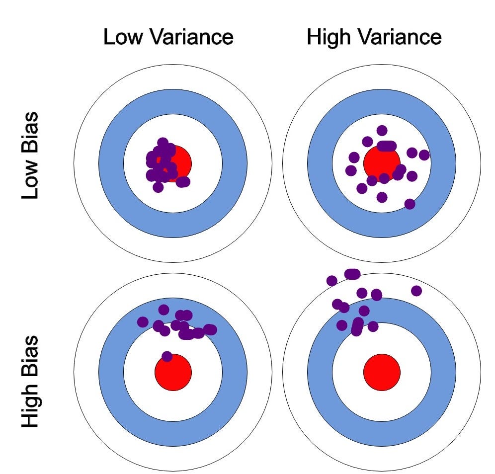
Regularization techniques almost always increase bias slightly in order to reduce variance significantly. The goal is a model that generalizes — one that captures the true structure of the task without memorizing the noise of the training set.
In vision and robotics, the practical question is: what is your deployment gap? The bigger the gap between your training data and your real-world distribution, the more aggressively you should regularize.
2. L2 regularization (weight decay)
What it does
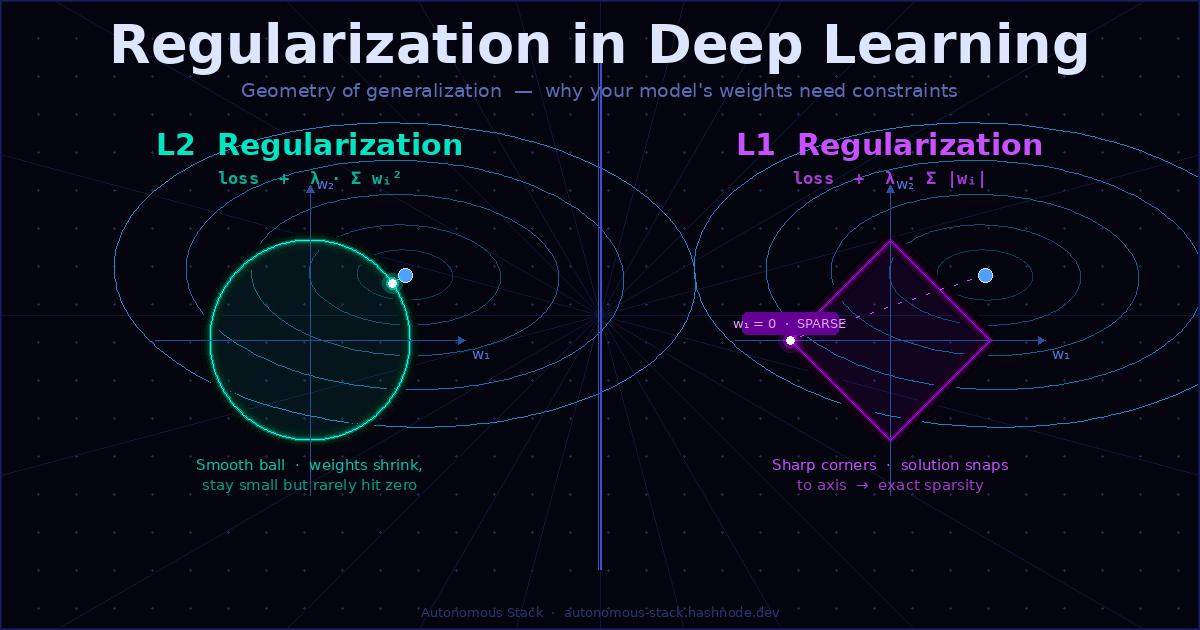
L2 regularization adds a penalty term to the loss function proportional to the squared magnitude of the weights:
$$\mathcal{L}{total} = \mathcal{L}{task} + \lambda \sum_{i} w_i^2$$
This discourages the network from assigning very large weights to any single feature. The optimizer is simultaneously minimizing the task loss and keeping weights small. The result is a smoother, more distributed representation.
Why it works
Large weights mean the network is making strong bets on specific features. In a vision model, that might mean it learned to key on a specific texture that appears in your training set but not in the real world. L2 forces the model to spread its bets.
In PyTorch
optimizer = torch.optim.AdamW(model.parameters(), lr=1e-4, weight_decay=1e-4)
AdamW is the correct way to apply weight decay with Adam. The original Adam with weight_decay parameter in PyTorch does not apply true L2 regularization — it conflates the decay with the gradient update. AdamW fixes this. Always use AdamW for vision transformers and modern architectures.
When to use it in robotics/CV
Almost always — it is the baseline regularizer. For ViT-based models (DINOv2, SAM, Depth-Anything), weight_decay=0.05 is the standard value from the original papers. For convolutional models, 1e-4 to 1e-2 depending on dataset size.
3. Dropout
What it does
During training, randomly zero out a fraction p of neuron activations at each forward pass. At inference, all neurons are active and their outputs are scaled by (1-p) to compensate.
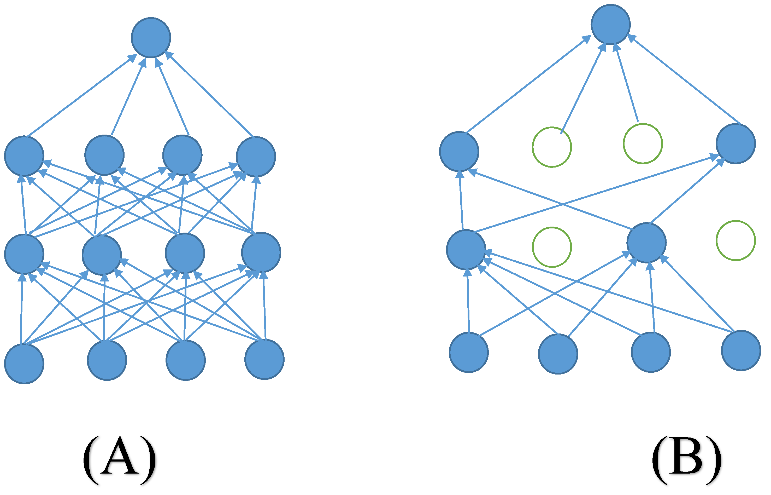
(A) - Full Layers No Dropout , (B) Some Neurons Dropped
import torch.nn as nn

class PerceptionHead(nn.Module):
    def __init__(self, in_features, num_classes):
        super().__init__()
        self.net = nn.Sequential(
            nn.Linear(in_features, 512),
            nn.ReLU(),
            nn.Dropout(p=0.3),
            nn.Linear(512, 256),
            nn.ReLU(),
            nn.Dropout(p=0.3),
            nn.Linear(256, num_classes)
        )

    def forward(self, x):
        return self.net(x)
Why it works
Dropout forces the network to learn redundant representations — no single neuron can rely on the presence of any other neuron. The result is an ensemble of many sub-networks trained jointly, which generalizes better.
DropPath for Vision Transformers
In ViT-based architectures, standard Dropout is less effective. The modern equivalent is DropPath (stochastic depth), which randomly drops entire residual paths rather than individual neurons:
from timm.models.layers import DropPath

class TransformerBlock(nn.Module):
    def __init__(self, dim, drop_path_rate=0.1):
        super().__init__()
        self.attn = Attention(dim)
        self.mlp = MLP(dim)
        self.drop_path = DropPath(drop_path_rate) if drop_path_rate > 0 else nn.Identity()
        self.norm1 = nn.LayerNorm(dim)
        self.norm2 = nn.LayerNorm(dim)

    def forward(self, x):
        x = x + self.drop_path(self.attn(self.norm1(x)))
        x = x + self.drop_path(self.mlp(self.norm2(x)))
        return x
DropPath is used in DINOv2, MAE, Swin Transformer, and virtually every modern ViT variant. If you are fine-tuning any of these for a robotics perception task, keep DropPath enabled during fine-tuning.
When to use it
Classification and detection heads: standard Dropout
0.2–0.5ViT/transformer backbones: DropPath, rate between
0.1–0.3Do not use Dropout in BatchNorm layers — they interact badly. If you are using BN, apply Dropout only after, never before.
4. Batch Normalization
What it does
Normalizes the activations across the batch dimension at each layer, then applies learned scale and shift parameters:
$$\hat{x}i = \frac{x_i - \mu\mathcal{B}}{\sqrt{\sigma_\mathcal{B}^2 + \epsilon}}, \quad y_i = \gamma \hat{x}_i + \beta$$
self.block = nn.Sequential(
    nn.Conv2d(64, 128, kernel_size=3, padding=1, bias=False),
    nn.BatchNorm2d(128),
    nn.ReLU(inplace=True)
)
Note bias=False — When BatchNorm follows a conv layer, the conv bias is redundant because BN shifts the output anyway.
Why it matters specifically in real-time or Edge applications
BatchNorm has a known problem in robotics: it behaves differently at train time and test time. At test time, it uses running statistics estimated during training. If your deployment distribution shifts — different lighting, different camera, different environment — those statistics become stale and your model quietly degrades.
This is not hypothetical.Lets Take drone example again - > In drone perception specifically, the same scene at 10m altitude and 50m altitude can have dramatically different image statistics. A model that normalizes using statistics from 10m footage will be miscalibrated at 50m .
The practical fix : consider Group Normalization or Layer Normalization for models that will face large distribution shifts at deployment, since they compute statistics per-sample rather than per-batch.
# GroupNorm — good alternative to BatchNorm for small batches or distribution shift
nn.GroupNorm(num_groups=32, num_channels=128)

# LayerNorm — standard in transformers, statistics per sample
nn.LayerNorm(normalized_shape=hidden_dim)
5. Data augmentation as regularization
Data augmentation is regularization. It artificially expands the training distribution, which is exactly what you need when your deployment distribution is unknown.
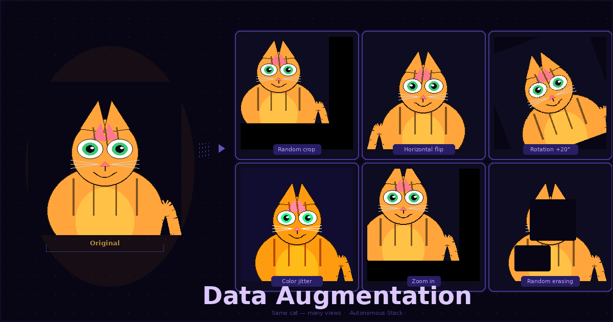
Standard augmentation for CV:
import torchvision.transforms as T
from torchvision.transforms import autoaugment

train_transform = T.Compose([
    T.RandomResizedCrop(224, scale=(0.6, 1.0)),
    T.RandomHorizontalFlip(),
    T.ColorJitter(brightness=0.4, contrast=0.4, saturation=0.4, hue=0.1),
    T.RandomGrayscale(p=0.2),
    T.GaussianBlur(kernel_size=23, sigma=(0.1, 2.0)), # Adds Gaussia Blur
    T.ToTensor(),
    T.Normalize(mean=[0.485, 0.456, 0.406],
                std=[0.229, 0.224, 0.225])
])
Robotics-specific augmentations worth knowing
Random erasing — simulates occlusion, which is extremely common in drone footage and warehouse environments:
T.RandomErasing(p=0.5, scale=(0.02, 0.2), ratio=(0.3, 3.3))
Motion blur — drones move fast. Your training images are sharp. Your deployment images are not:
import cv2
import numpy as np

def apply_motion_blur(image, kernel_size=15):
    kernel = np.zeros((kernel_size, kernel_size))
    kernel[int((kernel_size - 1) / 2), :] = np.ones(kernel_size)
    kernel /= kernel_size
    return cv2.filter2D(image, -1, kernel)
Perspective transforms — for ground robots and drones, the camera angle varies. Random perspective shift trains the model to be invariant to small viewpoint changes:
T.RandomPerspective(distortion_scale=0.3, p=0.4)
6. Mixup and CutMix
What they do
Mixup creates training samples by linearly interpolating between two images and their labels:
$$\tilde{x} = \lambda x_i + (1 - \lambda) x_j, \quad \tilde{y} = \lambda y_i + (1 - \lambda) y_j$$
CutMix cuts a rectangular patch from one image and pastes it into another, mixing labels proportionally to the patch area.
import numpy as np

def mixup_batch(images, labels, alpha=0.4):
    lam = np.random.beta(alpha, alpha)
    batch_size = images.size(0)
    index = torch.randperm(batch_size).to(images.device)

    mixed_images = lam * images + (1 - lam) * images[index]
    labels_a, labels_b = labels, labels[index]
    return mixed_images, labels_a, labels_b, lam

def mixup_criterion(criterion, pred, y_a, y_b, lam):
    return lam * criterion(pred, y_a) + (1 - lam) * criterion(pred, y_b)
Why does it help in robotics pipelines?
Mixup forces the model to produce smooth, interpolated predictions rather than sharp decision boundaries. In practice, this produces better-calibrated confidence scores — a model that says 0.85 confidence actually means something. For robotics systems where perception confidence feeds into planning and safety decisions, calibrated uncertainty is not optional.
CutMix is particularly effective for detection tasks because it encourages the model to use the entire image context rather than keying on a single dominant feature.
7. Early stopping
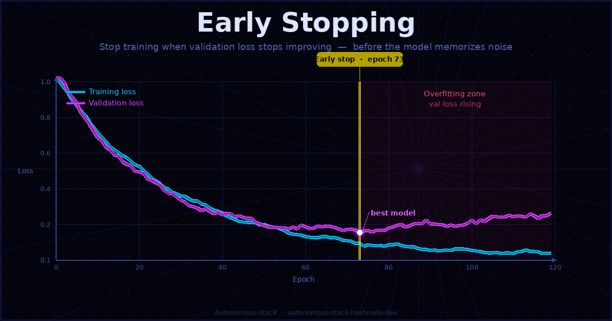
Simple idea worth understanding, Eraly Stopping means exactly the way it sounds - stop training when validation loss stops improving:
class EarlyStopping:
    def __init__(self, patience=10, min_delta=1e-4):
        self.patience = patience
        self.min_delta = min_delta
        self.counter = 0
        self.best_loss = float('inf')

    def __call__(self, val_loss):
        if val_loss < self.best_loss - self.min_delta:
            self.best_loss = val_loss
            self.counter = 0
            return False  # continue training
        else:
            self.counter += 1
            return self.counter >= self.patience  # stop if True

# Usage in training loop
early_stop = EarlyStopping(patience=15)

for epoch in range(max_epochs):
    train_one_epoch(model, train_loader, optimizer)
    val_loss = evaluate(model, val_loader)

    if early_stop(val_loss):
        print(f"Early stopping at epoch {epoch}")
        break
8. Label smoothing
Hard labels (0 or 1) push models toward overconfident predictions. Label smoothing replaces hard targets with soft targets:
$$y_{smooth} = (1 - \epsilon) \cdot y_{hard} + \frac{\epsilon}{K}$$
criterion = nn.CrossEntropyLoss(label_smoothing=0.1)
For robotics classification tasks — object class, terrain type, failure mode detection — you almost never have perfectly clean ground truth. Label smoothing acknowledges that uncertainty explicitly.
Putting it together: a practical prescription
| Scenario | Recommended regularization stack |
|---|---|
| Fine-tuning ViT for detection on drone footage | AdamW + weight_decay=0.05 + DropPath=0.2 + aggressive augmentation + Mixup |
| Training a small CNN on limited robotics data | L2 + Dropout 0.3 + ColorJitter + RandomErasing + early stopping |
| Depth estimation with distribution shift risk | GroupNorm instead of BatchNorm + heavy perspective augmentation + motion blur |
| Semantic segmentation on edge hardware | L2 + label smoothing=0.1 + CutMix + early stopping |
| Any model going to production from a small dataset | All of the above, dial back gradually as data grows |
The general rule: the smaller your dataset and the larger your deployment gap, the more regularization you need. If you are fine-tuning a large pretrained model (DINOv2, SAM, CLIP) on robotics-specific data, the backbone is already regularized by the pretraining. Focus your regularization effort on the task head.
What extras can you read next:
If this post was useful, these are the papers and resources worth going deeper on:
Dropout — Srivastava et al., 2014. arxiv.org/abs/1207.0580
DropPath / Stochastic Depth — Huang et al., 2016. arxiv.org/abs/1603.09382
Mixup — Zhang et al., 2018. arxiv.org/abs/1710.09412
CutMix — Yun et al., 2019. arxiv.org/abs/1905.04899
AdamW — Loshchilov & Hutter, 2019. arxiv.org/abs/1711.05101
Group Normalization — Wu & He, 2018. arxiv.org/abs/1803.08494
timm library — a PyTorch image model library with all modern regularization built in. github.com/huggingface/pytorch-image-models
The code in this post is available as a runnable notebook on GitHub — [link to repo -> here]. The next post covers normalization layers in depth: when BatchNorm silently breaks your model and what to replace it with.
About the author
- Autonomous systems engineer with 4+ years building production drone and land-based robotic platforms. I work on the full stack — computer vision, VIO, ROS2, edge AI, and cloud infrastructure — currently deploying on ModalAI VOXL2. Pursuing a master's in Autonomous Systems, focusing on VLA. I write about what I actually build and debug: real systems, real crashes, real code.
Comments
Join the discussionNo comments yet. Be the first to comment.